2 by 2 by 2 Tensors

We now study the case of \(2\times2\times2\) tensors over both the real and complex numbers. Our purpose is to give visualizations of theoretical work of others.

Visualizations over the Real numbers

We follow the work of Vin De Silva and Lek-Heng Lim in [DES-LIM2008], although several of these results appeared earlier in [KRUSKA1989]. They show that all \(2\times2\times2\) tensors are in \(S_3\) but both \(S_2\) and \(S_3\setminus S_2\) have positive volume. The tensors in \(S_3\setminus S_2\) can be divided into the cases \(D_3\) and \(G_3\).

Degenerate Separation Rank 3

The class \(D_3\) consists of tensors not in \(S_2\) that are a limit of tensors in \(S_2\). The existence of tensors in \(D_3\) shows that \(S_2\) is not a closed set. A representative element of \(D_3\) is

\[D_3 = [1,0]\otimes[1,0]\otimes[1,0] + [1,0] \otimes [0,1]\otimes [0,1] + [0,1]\otimes [1,0]\otimes [0,1] \,,\]

which can also be viewed as

\[\begin{split}D_3 = \left[\begin{array}{cc}1&0\\0&0\end{array}\right]\otimes[1,0] + \left[\begin{array}{cc}0&1\\1&0\end{array}\right]\otimes [0,1] \,.\end{split}\]

Using the plane defined by the three tensors

\[\begin{split}T_1&= [1,0]\otimes [1,0]\otimes [1,0]\,, \\ T_2&=[1,0] \otimes [0,1]\otimes [0,1]\,, \quad\text{and}\\ T_3&=[0,1]\otimes [1,0]\otimes [0,1]\,,\end{split}\]

the point \(D_3\) is in their center. Since these three tensors are in \(S_1\), any tensor on the line connecting any two of them is in \(S_2\). These lines help us identify the three tensors in the visualization, and thus help approximately locate the \(D_3\) tensor.

Plotting \(S_2\) in this way, we obtain the visualization

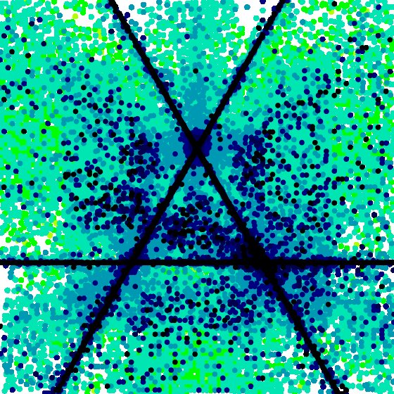
[data file 2x2x2pr2D3.dat] Notice that we obtain black points near \(D_3\), and this lack of a void validates the result that there are tensors in \(S_2\) near \(D_3\). It does not allow us to distinguish points in \(D_3\) from points in \(S_2\).

General Separation Rank 3

The class \(G_3\) consists of tensors not in \(S_2\) that are not a limit of tensors in \(S_2\). A representative element of \(G_3\) is

\[G_3 = [1,1]\otimes[0,1]\otimes[0,1] + [1,-1]\otimes[1,0]\otimes[1,0] + [0,1]\otimes [1,1]\otimes [1,-1] \,,\]

which can also be viewed as

\[\begin{split}G_3 = \left[\begin{array}{cc}1&0\\0&1\end{array}\right]\otimes[1,0] + \left[\begin{array}{cc}0&1\\-1&0\end{array}\right]\otimes [0,1] \,.\end{split}\]

Using the plane defined by the three tensors

\[\begin{split}T_1&=[1,1]\otimes[0,1]\otimes[0,1] \,,\\ T_2&=[1,-1]\otimes[1,0]\otimes[1,0] \,,\quad\text{and}\\ T_3&=[0,1]\otimes [1,1]\otimes [1,-1] \,,\end{split}\]

the point \(G_3\) is in their center. Since these three tensors are in \(S_1\), any tensor on the line connecting any two of them is in \(S_2\). These lines help us identify the three tensors in the visualization, and thus help approximately locate the \(G_3\) tensor.

Plotting \(S_2\) in this way, we obtain the visualization

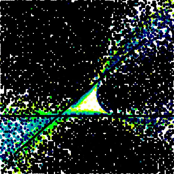
[data file 2x2x2pr2G3.dat] We obtain black points everywhere outside of the triangle, and part of the region inside of the triangle. However, near \(G_3\) there is a distinct void, indicating that this tensor cannot be approached as a limit of tensors in \(S_2\).

We also note that we used only one-third the points to make this visualization as compared to the \(D_3\) visualization, and yet obtained more black points. This indicates that the ALS routine had more difficulty on the tensors in the \(D_3\) plane, perhaps because they are only limit points of \(S_2\).

Random Example

Randomly choosing \(T_1\), \(T_2\), and \(T_3\), we obtained a visualization

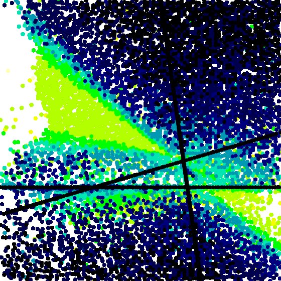
[data file 2x2x2pr2random.dat] In this visualization we see both black regions and voids, suggesting that it is relatively easy to hit both types of behaviors.

Visualizations over the Complex numbers

Over the complex numbers the \(2\times2\times2\) tensors in \(G_3\) have only rank 2 and collapse into \(S_2\) (p.1119, [DES-LIM2008] ). We illustrate this by considering the \(G_3\) tensor defined above. Using the complex line defined by the two tensors

\[\begin{split}T_1&=[1,1]\otimes[0,1]\otimes[0,1]+[1,-1]\otimes[1,0]\otimes[1,0] \,,\quad\text{and}\\ T_2&=[0,1]\otimes [1,1]\otimes [1,-1] \,,\end{split}\]

the point \(G_3\) is the (real) midpoint of the line. Plotting \(S_2\) in this way on \([-1,2]\times[-i,i]\), we obtain the visualization

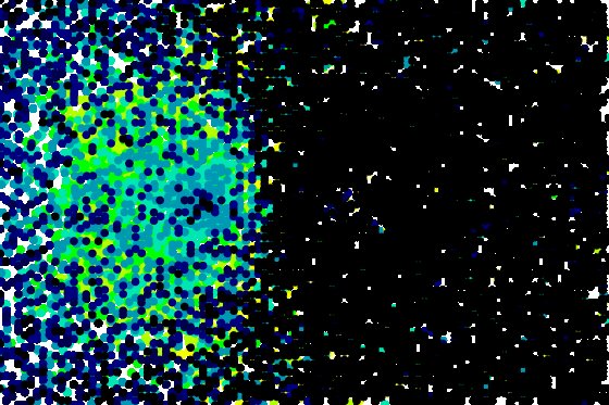
[data file 2x2x2pr2G3C.dat] We obtain black points everywhere, indicating that \(G_3\) is in \(S_2\) over the complex numbers (prehaps as a limit point). The ALS routine had more trouble finding black points in the left half of the visualization, which is closer to \(T_2\). This is counterintuitive, since \(T_2\) is only rank 1 whereas \(T_1\) is rank 2.

However, tensors in \(D_3\) still have rank 3. Since they are (still) limits of tensors in \(S_2\), our visualization will not be able to detect them.