2 to the 9th Tensors
We now study the case of tensors with \(d=9\) and \(M=2\). At worst, the maximum rank is \(2^8=256\). By unfolding such a tensor to a \(2^4\times 2^5\) matrix, one can see that rank \(2^4=16\) is definitely achievable.
Visualizations over the Real numbers
A Specific Example
We are interested in analyzing the tensor
which has nominal rank 9. Consider the tensor-valued function
and notice that the derivative of \(G(t)\) at 0 is \(L_9\), i.e. \(G'(0)=L_9\). Since
we see that \(L_9\) is a limit of rank 2 tensors. (To avoid loss-of-precision errors due to cancellation, larger rank is needed; see [BEY-MOH2005].)
To visualize \(L_9\), we choose
so that \(L_9\) will be in the center of these three tensors. Since these three tensors are in \(S_3\), any tensor on the line connecting any two of them is in \(S_6\), and a tensor in the plane is generically in \(S_9\).
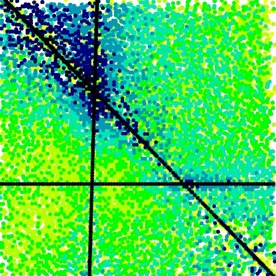
We first produce a visualization of \(S_2\) on \([-1,2]\times[-1,2]\), and obtain
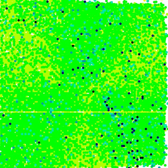
[data file 2to9pr2L9.dat] Black points are scattered sparsely on the visualization, but without apparent voids. It appears that the ALS routine had some difficulty (with its fixed number of iterations). There is a light horizontal streak along the line connecting \(T_1\) to \(T_3\) of unknown cause, probably a numerical artifact.
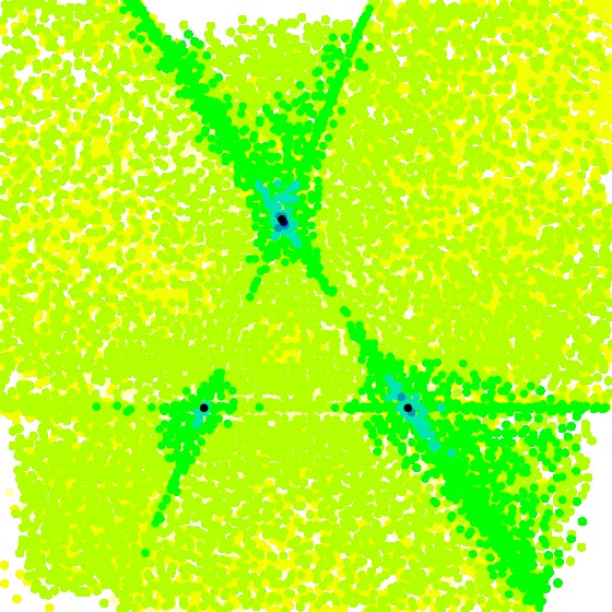
Next, we produce a visualization of \(S_3\), and obtain
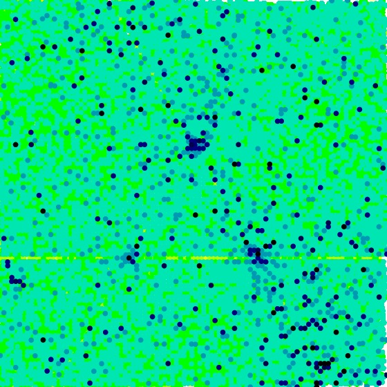
[data file 2to9pr3L9.dat]
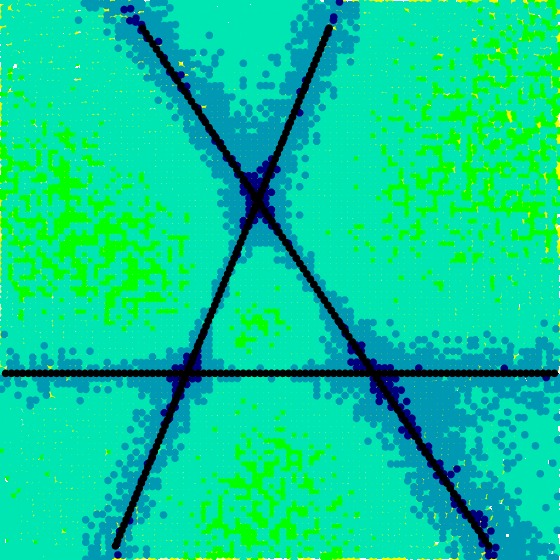
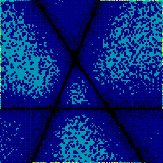
Next, we produce a visualization of \(S_6\), which includes the lines connecting any two of our base tensors, and obtain
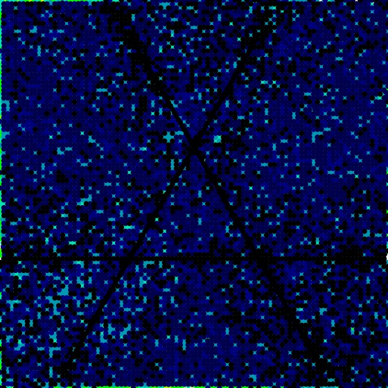
[data file 2to9pr6L9.dat]
A Random Example
To complement the specific example above, we choose \(T_1\), \(T_2\), and \(T_3\) randomly in \(S_3\). Since these three tensors are in \(S_3\), any tensor on the line connecting any two of them is in \(S_6\), and a tensor in the plane is generically in \(S_9\).
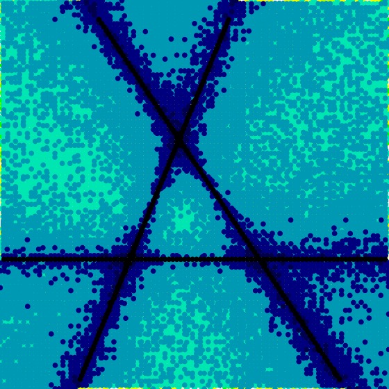
We first produce a visualization of \(S_3\) on \([-1,2]\times[-1,2]\), and obtain
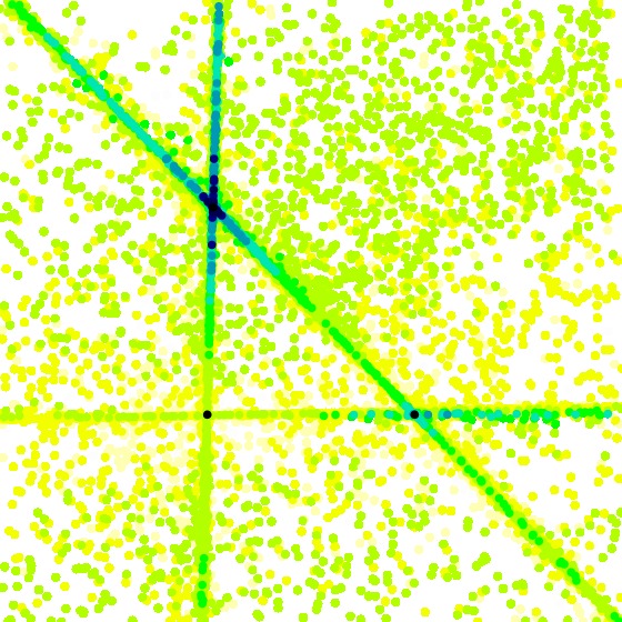
[data file 2to9pr3random.dat] Next, using the same set of random \(T_1\), \(T_2\), and \(T_3\), we produce a visualization of \(S_6\), and obtain
[data file 2to9pr6random.dat] Since in neither case do we find any unexpected black points, we conclude that the specific example above is not typical.
A Second Random Example
To complement the specific example above, we choose \(T_1\), \(T_2\), and \(T_3\) randomly in \(S_{16}\). Since these three tensors are in \(S_{16}\), any tensor on the line connecting any two of them is in \(S_{32}\), and a tensor in the plane is generically in \(S_{48}\).
We first produce a visualization of \(S_{16}\) on \([-1,2]\times[-1,2]\), and obtain
[data file 2to9pr16random2.dat] Next, using the same set of random \(T_1\), \(T_2\), and \(T_3\), we produce a visualization of \(S_{32}\), and obtain
[data file 2to9pr32random2.dat]
Next, using the same set of random \(T_1\), \(T_2\), and \(T_3\), we produce a visualization of \(S_{40}\), and obtain
[data file 2to9pr40random2.dat]
Finally, we produce a visualization of \(S_{48}\), which should be black, and obtain
[data file 2to9pr48random2.dat] Although we do not obtain black, we do obtain dark blue, indicating that the fitting is working fairly well.
The first time we ran the tests for this example, we used the ALS algorithm at fixed rank rather than growing the rank (see ALS Performance Notes). That algorithm performed much worse, as illustrated in the Section A note on ALS failure.