If you have difficulty accessing these materials due to visual impairment, please email me at mohlenka@ohio.edu; an alternative format may be available.
We are studying approximations for tensors \(T\) of the form
\[
T(j_1,j_2,\dots,j_d)
\approx
G(j_1,\dots,j_d)
=\sum_{l=1}^{r} G^l(j_1,\dots,j_d)
=
\sum_{l=1}^r \prod_{i=1}^{d} G_i^l(j_i)
\quad\text{for}\quad j_i=1,2,\dots,M_i
\,,
\]
or equivalently
\[
T
\approx
G
=\sum_{l=1}^{r} G^l
=
\sum_{l=1}^r \bigotimes_{i=1}^{d} G_i^l
\,,
\]
where \(d\) is the "dimension" (number of variables).
As a particular test case, we consider the rank-2 tensors
\[
T = \left(1+2 z\cos^d(\phi)+z^2\right)^{-1/2}
\left(\bigotimes_{i=1}^{d} \mathbf{u}(0)
+z\bigotimes_{i=1}^{d} \mathbf{u}(\phi)\right)
\,,
\]
where
\( 0\le \phi \le \pi/2 \) (indirectly) controls the angle
between the two summands,
\(|z|\le 1\) controls the relative size and direction of the
two summands, and
the scalar \(\left(1+2 z\cos^d(\phi)+z^2\right)^{-1/2}\) makes
\(T\) have norm 1.
We measure the approximation error by
\[
E_\lambda(G)
=E_\lambda(G^1,\dots,G^r)
=\|T-G\|_2^2 +\lambda\sum_{l=1}^r \|G^l\|_2^2
\]
for some \(\lambda \ge 0\).
Approximation with Rank \(r=1\)
If we choose \(r=1\), then our approximation can be written as
\[
G = a \bigotimes_{i=1}^{d} \mathbf{u}(\alpha_i)
\,.
\]
Given the angles \(\{\alpha_i\}_{i=1}^d\), the optimal value for
the scalar
\(a\) can be easily determined, so we assume \(a\) is set
optimally.
We will consider the symmetric case, when \(\alpha_i=\alpha\)
for all \(i\).
We will visualize two aspects of this approximation. In both
cases we choose values for \(d\), \(z\), and
\(\lambda\) and plot with \(0\le\phi\le\pi/2\) on the horizontal axis
and \(-\pi/2 \le \alpha-\phi/2 \le \pi/2\) on the vertical axis.
The downward and upward slanted lines give the positions of
the first and second summands in the target.
On the left, we plot the error \(E_\lambda(G)\).
On the right, we plot the stability of the gradient flow on
the symmetric set \(\alpha_i=\alpha\). Values bigger than 1/2
mean that the symmetric state is unstable and flow along the
negative gradient will amplify asymmetry.
\(d=\)
\(\lambda=\)
\(z=\)
Approximation with Rank \(r=2\)
If we choose \(r=2\), then our approximation can be written as
\[
G = a \bigotimes_{i=1}^{d} \mathbf{u}(\alpha_i)
+ b \bigotimes_{i=1}^{d} \mathbf{u}(\beta_i)
\,.
\]
Given the angles \(\{\alpha_i\}_{i=1}^d\) and
\(\{\beta_i\}_{i=1}^d\), the optimal values for the scalars
\(a\) and \(b\) can be easily determined, so we assume \(a\)
and \(b\) are set optimally.
We will consider the symmetric case, when \(\alpha_i=\alpha\)
and \(\beta_i=\beta\) for all \(i\).
We will visualize two aspects of this approximation. In both
cases we choose values for \(d\), \(\phi\), \(z\), and
\(\lambda\) and plot with
\(-\pi/2 \le \alpha-\phi/2 \le \pi/2\) on the horizontal axis
and \(-\pi/2 \le \beta-\phi/2 \le \pi/2\) on the vertical
axis.
The horizontal and vertical lines indicate the positions of
the first and second summands in the target, at angles \(0\)
and \(\phi\).
On the left, we plot the error \(E_\lambda(G)\).
On the right, we plot the stability of the gradient flow on
the symmetric set \(\alpha_i=\alpha\) and \(\beta_i=\beta\).
Values bigger than 1/2
mean that the symmetric state is unstable and flow along the
negative gradient will amplify asymmetry.
\(d=\)
\(\lambda=\)
\(z=\)
\(\phi=\)
Approximation with Rank \(r=3\)
If we choose \(r=3\), then our approximation can be written
as \[ G = a \bigotimes_{i=1}^{d} \mathbf{u}(\alpha_i) + b
\bigotimes_{i=1}^{d} \mathbf{u}(\beta_i) + c
\bigotimes_{i=1}^{d} \mathbf{u}(\gamma_i) \,. \] Given the
angles \(\{\alpha_i\}_{i=1}^d\), \(\{\beta_i\}_{i=1}^d\), and
\(\{\gamma_i\}_{i=1}^d\), the optimal values for the scalars
\(a\), \(b\), and \(c\) can be easily determined, so we assume
they are set optimally. We will consider the symmetric case,
when \(\alpha_i=\alpha\), \(\beta_i=\beta\), and
\(\gamma_i=\gamma\) for all \(i\). We plot with \(-\pi/2 \le
\alpha-\phi/2 \le \pi/2\) on one axis, \(-\pi/2 \le \beta-\phi/2
\le \pi/2\) on the second axis, and \(-\pi/2 \le \gamma-\phi/2
\le \pi/2\) on the third axis; by symmetry it does not matter
which axis is which. The thin white tubes mark
\((\alpha,\beta,\gamma)=(0,\phi,\text{any})\) and its
permutations, where two terms in the approximation match the two
terms in the target.
Each video shows the contours of \(E_\lambda(G)\) as the
value moves from 1 to 0. The video then rotates to show the
same moving contours from a different angle. Note that when
the contour moves slowly it indicates large gradient so the
gradient flow would move quickly. When the contour moves
quickly, the gradient flow would move slowly.
Choosing \(d=6\), \(z=1\), and \(\lambda=0\)
\(\phi=\pi/2\)
\(\phi\approx 0.27\pi\)
\(\phi=\pi/8\)
Choosing \(d=6\), \(z=1/2\), and \(\lambda=0\)
\(\phi=\pi/2\)
\(\phi\approx 0.27\pi\)
\(\phi=\pi/8\)
Choosing \(d=6\), \(z=-1/2\), and \(\lambda=0\)
\(\phi=\pi/2\)
\(\phi\approx 0.39\pi\)
\(\phi=\pi/8\)
Choosing \(d=6\), \(z=-1\), and \(\lambda=0\)
\(\phi=\pi/2\)
\(\phi\approx 0.39\pi\)
\(\phi=0\)
Laplacian Cartoon
When \(z=-1\), plugging in
\(\phi=0\) yields an indeterminate form \(0/0\), but we can
compute the limit \[ \lim_{\phi\rightarrow 0^+}
\left(2-2\cos^d(\phi)\right)^{-1/2} \left( \bigotimes_{i=1}^{d}
\mathbf{u}(0) -\bigotimes_{i=1}^{d} \mathbf{u}(\phi) \right)
=\lim_{\phi\rightarrow 0^+} \left(2-2\cos^d(\phi)\right)^{-1/2}
\left(v(0)-v(\phi)\right) \,, \] and find (after some work) that
it equals \[ L=\frac{-1}{\sqrt{d}}\sum_{j=1}^{d}
\left(\bigotimes_{i=1}^{j-1}\mathbf{e}_1\right) \otimes
\mathbf{e}_2 \otimes
\left(\bigotimes_{i=j+1}^{d}\mathbf{e}_1\right) \,. \] Although
\(L\) is rank \(d\), it is the limit of rank-2 tensors, which
makes it a strange and interesting example. It has the same
structure as the \(d\)-dimensional Laplacian, which also makes it
important.
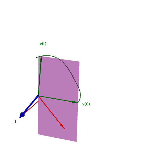
Below is an attempt to illustrate how such a strange thing can
happen. The blue vector shows \(L\) and the
green vector labeled v(0) shows the location of the fixed
vector \(v(0)\), which is orthogonal to \(L\). The green curve
gives the possible positions of \(-v(t)\) as \(t\) varies and the
green vector labeled -v(t) shows the location of the
vector \(-v(t)\) for the current \(t\). The red vector shows
\(T\) for the current \(t\).
The purple plane shows
the span of \(\{v(0),v(t)\}\) and the red segment shows the
(error of the) orthogonal projection of \(L\) onto this
span; these were not described above but give another way to
think about this example.
As \(t\rightarrow 0^+\) the error goes
to zero but if \(t=0\) then the span collapses to a line
orthogonal to \(L\) and so the best approximation of \(L\) is 0.